Juvenile White Shark Behavior and Biology
The CSULB Shark Lab has been studying the juvenile white sharks found off southern California for 16 years, in an effort to learn more about their behavior, migration patterns, and biology. We share this information with lifeguards, regulatory agencies, and the general public in an effort to improve safety for people, while also helping to improve management strategies for this species. This work began as a collaboration with Monterey Bay Aquarium with the goal of understanding the behavior and environmental preferences of juvenile white sharks. As the population continues to grow, we are also seeing and tagging more adult white sharks around the offshore islands (Catalina, Northern Channel Islands), Santa Barbara, and San Luis Obispo Counties.
What is a White Shark (aka Great White Shark)
The white shark (Carcharodon carcharias) is a member of the Lamnidae family, a group of sharks known for their streamlined shape that makes sharks in this family highly efficient swimmers. Close relatives of the white shark include the salmon shark (Lamna ditropis), mako sharks (Isurus spp.), and the porbeagle shark (Lamna nasus).
White sharks are a slow-growing species and can live up to 70 years or more. They reach an average length of 14-16 ft. (4.3-4.5 m), with females of the species typically growing larger. Some of the largest white sharks on record have reached approximately 20 ft. (6.1 m) in length. Like all fish, white sharks continuously grow in length over their lifetime, but while growth in length slows down, they tend to increase in girth as they age.

There are genetically distinct populations of white sharks distributed globally in temperate and subtropical waters. These populations spend their time migrating between offshore feeding grounds and coastal-aggregation hotspot areas throughout the year. Juveniles tend to be found nearshore, which suggests that birthing occurs in coastal waters and young white sharks use these areas as nurseries.
White sharks inhabit coastal and oceanic environments, and their movements range in depth. They travel from the surface (dorsal fin breaking the surface) to depths of over 3,280 ft. (1000 m), but have been known to make deeper dives of nearly 4,200 ft. (1280 m) deep. The purpose of these dives is likely for feeding, but little is known about their activity on these dives.

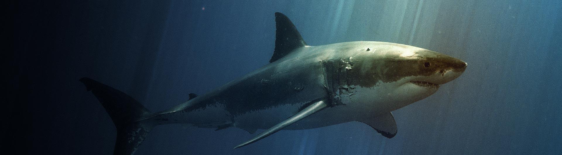
White sharks are characterized by having a sharply pointed snout and 5 gill slits on each side of their body. They have a large, stiff, lunate-shaped tail, large pectoral fins, and a triangular dorsal fin that aids with stabilization and maneuverability while swimming.
White sharks have a tapered grouping of muscles and connective tissue near the tail, known as the caudal peduncle, which provides the necessary power for the white shark's lunate (crescent shaped) caudal fin. The caudal peduncle helps propel them efficiently through the water. White sharks also possess one lateral keel that improves the stability of the caudal fin and minimizes drag over the part of the body that drives the caudal fin.

White sharks are typically dark gray, bluish-gray, or brown on the upper surfaces of their body and white underneath. This pattern of coloration is commonly described as countershading.
Countershading is a form of camouflage that allows the shark to avoid detection by its prey from above or below, and it has evolved in many other animals including fishes, marine mammals, and penguins. Countershading also allows a white shark to sneak up on its prey from below.

How can you tell if the dorsal fin you're seeing breaking the surface is from a dolphin or a shark? Visit our section on Staying Safe at the Beach to learn more!
White Shark Nurseries in Southern California
In recent years, an increasing number of juvenile white sharks have been observed near many southern California beaches, especially during the summer and fall months. These months typically coincide with an increase in human ocean-recreation, as well. Many of these white sharks are newborns and/or young individuals that use the beaches as nursery habitat (i.e. habitat where the young of a species grow up).
For these young white sharks, southern California beaches provide the ideal nursery habitat for various reasons:
- Beaches have warmer water
- Plenty of easy to capture food (stingrays, fish, squid)
- Safety from predators like adult white sharks, large mako sharks and orca

Female white sharks give birth to live young, and when white sharks are first born, they are 4-5 ft. (1.5 m) in length and are called the young of the year (YOY - so less than 1 year old). The mother does not provide any parental care, and the newborns are fully independent the moment they are born. While no one has ever seen a white shark giving birth, and we do not know where birthing actually occurs, it is suspected that birthing occurs in deeper water, and the newborns move towards the shallower shoreline waters seeking protection and warmth.

While it is difficult to determine how fast young white sharks can grow, captive studies at Monterey Bay Aquarium and recapture of juvenile sharks in the field, suggests that young individuals can grow about 12" (25 cm) per year for their first 5-6 years. Some researchers group young white sharks into these size categories - neonate, YOY, and juvenile. A white shark between 6-10 ft. (less than 3.0 m) in length is considered a juvenile white shark (JWS). These size classes (neonate, YOY, and juvenile) will utilize a nursery habitat until they are big enough to transition to their adult diet and habitat.

Two nursery areas have been identified for white sharks in the Eastern North Pacific Ocean: southern California and Vizcaino Bay, Baja CA, Mexico.

Depending on water temperature, YOY and JWS are most common along southern California beaches from April-October, and in the late fall, YOY sharks migrate south to Vizcaino Bay, Baja CA, Mexico. The next spring, some individuals will migrate north to SoCal nursery areas.
Within the nursery habitat, there are seasonal hotspots where YOY and JWS are most commonly found. These hot spots can vary from year-to-year, and they may frequent nursery hot spots for several years before eventually moving to adult aggregation sites (e.g., Monterey Bay, Ano Nuevo, Northern Channel Islands, Guadalupe Island).

We do not yet fully understand what makes a good hot spot area for YOY and JWS and how this changes over time, but the CSULB Shark Lab has several projects underway to further investigate habitat preferences, feeding behavior, and migration patterns.

Frequently-Asked Questions
Tap on a question to read the answer.
(Do juvenile white sharks choose certain nursery hotspot beaches because its warmer?)
JWS are one of the few warm-bodied sharks that use nearshore nursery habitats; however, juveniles are thought to be too small to maintain their body temperature efficiently. Because of this, they may seek out warmer water and form lose aggregations with other individuals.
Video 1: Shark aggregation.
We can monitor sharks through tagging and tracking.
Tagging
Sharks are tagged with acoustic transmitters, which use sound waves to transmit a unique ID. Some of the tags have a pressure and temperature sensor on them, which provides extra information on the depth and temperature that the shark is swimming at.
Since JWS can range in size from 4-10 ft (1-3 m), if they are small enough, we can catch them using a method called strike netting. Strike netting allows us to surgically implant a tag, record the individual's length and girth, and identify if it is a male or female.


However, if the shark is either too large, or the water conditions are not optimal to catch the shark, we tag the sharks using a method called jab tagging. There are several steps to this process. First, we find a shark that is swimming near the surface and position the boat as close as we can behind it.

To determine if it is male or female, we use a GoPro camera attached to the end of a long pole to take video of the underside of the shark.

After we have identified the sex of the shark, we dart an acoustic tag into the shark's back near the dorsal fin. To do so, we use a modified pole spear with the transmitter fixed to the end.
Video 2: Dr. Lowe, director of the Shark Lab, jab tagging a juvenile white shark.
Tracking
We use acoustic receivers placed along the seafloor to listen for the acoustic transmitters on the sharks, which record the date, time, and ID of the shark that swims within a certain range. These receivers can listen for transmitters in 360° 24/7 and can detect transmitters at a range depending on the power of the transmitter (100-700 yards away). While we have a larger network of receivers from central California down to San Diego and into parts of Baja California, in the aggregation sites, these receivers are placed in a dense array ~500 yards apart. Since these receivers store collected detection data, a team of scuba divers must dive to retrieve them so they can be downloaded data on the surface. Then, we can determine how many sharks were detected, and when the sharks were present near the receiver.


In the aggregation site (i.e. hotspot), if 3 or more of the receivers detect the same shark at about the same time, we can determine exactly position using triangulation. This allows us to get a better idea of how the sharks are using the space and how they respond to changing environmental conditions like water temperature.
Video 3: In this animation, individual tagged sharks are represented by a different color. Each receiver is represented by a white dot. You can see how sharks use different areas at this nursery site over a one week period.
Measuring Water Temperature at a Fine Scale
To figure out if specific temperatures influence how juvenile white sharks are moving within the beach site, and how long they remain at that site, we monitor temperature throughout the water column on a continuous scale. We do this using temperature loggers, which record the water temperature every hour. Some loggers are placed on the sea surface, and some are placed on the sea floor at each receiver location. This allows us to see how temperature changes over the entire deployment period of our receiver array, both at the surface and at depth.
Video 4: In this temperature animation you can see how much water temperature can change within a relatively small area over the course of a tide. Since sharks are responding changes in the environment around them, we can use these data to figure out how water temperature may influence where they spend their time, how the regulate their energy consumption and when they migrate.
To more closely monitor temperature across the entire water column, we also use an autonomous underwater vehicle (AUV). The AUV is used to determine if there are any changes in temperature on a smaller spatial scale, that the temperature loggers placed ~500 yards apart on the receivers may have missed.

Video 5: AUV starting a mission.
Since we run the AUV through the habitat where the sharks aggregate, we occasionally get sharks that are curious of this odd noisy yellow torpedo, and some have even taken a bite - like a dog playing with a toy.

In addition to measuring water temperature in 3D, the AUV also measures: salinity, depth, amount of chlorophyll (representative of phytoplankton), dissolved oxygen (DO), and turbidity.

Once we know the positions from the acoustic receiver array and corresponding 3D temperature maps of the area, we use this data to determine if sharks are tracking particular patches of warm water. Preliminary results indicates that water temperature does influence how long JWS will stay at the aggregation site. When temperatures drop too low and stay low (below 60° F), they will begin their search for warmer water elsewhere, usually to the south.
Previous studies on the diet of YOY and JWS from other populations have revealed young white sharks primary feed on bottom-dwelling marine organisms such as stingrays, bat rays, small fish, crabs, and squid, which are abundant nearshore.
In southern California, we have found round stingrays, bat rays, and California halibut in the stomachs of dead sharks we have examined. Round stingrays are small, bottom-dwelling elasmobranchs, or cartilaginous fish, and are distributed in the North Pacific Ocean from Panama to Humboldt, Northern California and are particularly abundant along southern California beaches. Juveniles can be found in bays and estuaries, and adult round stingrays are often found in nearshore sandy habitats along the coast.

Bat rays are another elasmobranch (cartilaginous fish) species that juvenile white sharks like to eat. They find rest and refuge in sandy areas, where they display little activity, and they forage for food in rocky reef habitats. Bat rays are distributed from the Gulf of California, Mexico, to the Oregon Coast.

The California halibut is a bottom-dwelling teleost, or bony fish, with large teeth. They are a type of flounder distributed from Baja California to Washington

Figure 23 Reference: http://www.csun.edu/~nmfrp/californiahalibut.html
Yellowfin croaker are teleosts (bony fish) that swim in the water column. They are often found in nearshore areas along sandy beaches, and they are distributed from the Gulf of California, Mexico, to Point Conception, California.

Figure 24 Reference: https://marinespecies.wildlife.ca.gov/yellowfin-croaker/
Trying to figure out what sharks eat is actually quite challenging. In the past, the way we learned about what sharks ate was to catch and kill them, cut open their stomachs to see what they had recently eaten. 10,000s of sharks around the world have been sampled this way, which is a pretty destructive way to answer the question. In some cases, we have observed juvenile white sharks feeding on stingrays from drones, but we're missing many feeding events, likely on other species, we need another tool for determining what they are eating. A new, less invasive method involves tracking nutritional signals known as stable isotopes found in the sharks' tissues incorporated from the foods they eat.
An atom's nucleus is made out of protons and neutrons. In nature, we can find molecules from the same element (e.g., carbon, nitrogen, hydrogen, oxygen, sulfur) with the same number of protons, but different number of neutrons. The sum of protons and neutrons gives the atomic mass of the molecule. Consequently, we can find heavy and light isotopes in natural environments. The extra number on neutrons in heavy isotopes make the chemical bonds in these molecules stronger. Thus, heavy isotopes are stable, which means they do not decay into other elements, they get incorporated into the food chain, and can be trackable within living and non-living organisms.

Figure 25 Reference: https://theplosblog.plos.org/2012/12/so-you-wanna-be-a-paleoecologist-p…
The stable isotopes most commonly used to study sharks' diet are carbon and nitrogen, which become the building blocks for new tissues in the consumer's body.
Nitrogen is an important nutrient that helps regulating primary productivity in both aquatic and terrestrial ecosystems. Microbially-driven processes such as, nitrogen fixation, nitrification, and denitrification, constitute the bulk of nitrogen transformations. Once nitrogen is fixed through these biochemical processes, it becomes available for plants.
Plants use nitrogen to maximize growth and make their own food through photosynthesis. Similarly, carbon enters the food chain when carbon dioxide is used in photosynthesis. As a consequence, both elements get incorporated into herbivores' tissues as they feed on plants, and in carnivores' tissues as they feed on smaller animals.
When sharks feed, they get carbon and nitrogen isotopes from their prey. As a result, both elements get incorporated into the sharks' tissues (e.g., muscle and blood). Both, heavy and light isotopes get incorporated into the consumers' tissues, but lighter isotopes tend to be used on biochemical reactions or excreted by the animal. Thus, the heavy isotopes (e.g., 13C and 15N) are recruited into new tissues. This phenomenon is known as isotope fractionation. Nitrogen isotope fractionation increases at each trophic level. This is known as nitrogen enrichment. This means that sharks feeding on bigger or larger prey, that will likely provide more protein and nutritional value, will exhibit higher nitrogen enrichment. Saying this, nitrogen is a good indicator of the trophic position of the shark. In other words, we can estimate how low or high in the food chain a shark is feeding at.
Carbon isotope fractionation exhibits little variation across trophic levels. Nonetheless, carbon fractionation is highly dependent on the primary productivity and the type of photosynthetic pathway dominating a ecosystem. In other words, the more abundant type of primary producers at a specific habitat type (e.g., corals, kelp forest, phytoplankton). Because carbon isotopic signatures remain constant across the food chain but vary at the base of the food chain, carbon can be used like a GPS to identify potential habitat types being used by the shark to hunt and feed (e.g., coastal or offshore; freshwater or saltwater zones).

But, each tissue provides different clues to solve the mystery of a shark's diet.
Solving the Mystery
Looking at carbon and nitrogen ratios from different tissues is like reading the diet journal of a shark, because different tissues incorporate isotopes from recent meals at different rates. For example, blood incorporates carbon and nitrogen isotopes faster than muscle. This means that different shark tissues will assimilate preys' isotopes at different rates. Consequently, multiple tissues may provide information on what sharks have been eating over various periods of time.
Ratios of carbon and nitrogen from blood samples provide insights into the type of food consumed by the shark, weeks/months before the date the sample was taken. Stable isotope ratios from a muscle sample provide information of what the shark ate a year prior the sampling date. By looking at stable isotopes from different tissues we can get insights into dietary changes.

We can get small muscle samples from free-swimming white sharks by sneaking up on them from a boat using a drone to spot and track them. Then we can use a modified pole spear with a biopsy punch attached.
Video 6: Shark Lab graduate student Yamilla Samara taking a muscle sample from a juvenile white shark.

When sharks are caught either incidentally by commercial fishers or deliberately by our team using strike netting (explained above) we can collect blood samples from the caudal vein by using a syringe and needle.

Figuring out what sharks are eating is important, but learning what they prefer requires knowing what food is available to them. This too can be challenging because some prey may be patchy in their distribution, some may move a lot, and some may learn to avoid predators. So, to determine if juvenile white sharks are selecting certain nursery areas because there are more prey, we're trying to count potential shark prey – the beach buffet.
Beach seines are long nets that we use to catch animals that are near the wave break. A group of 7-8 people is needed to walk the net and pull it back to shore.


Anotter trawl is a cone-shaped net that we use to sample animals that are deeper in the water column. This allow us to sample potential prey species that can't be caught with a beach seine.


You Can't Catch Everything
In order to count how many individual prey items there are, we use a variety of methods! We can use beach seines and otter trawls (see above) to capture prey species and count how many individuals there are.
We also use baited underwater remote videos (BRUVs) to estimate the abundance (number of individuals present) of some prey species. BRUVs use just a little bit of squid in mesh container to lure fish to the camera station. Each BRUV has a GoPro camera located 3' above the seafloor and one right on the seafloor so we can see bottom-dwelling fish and those that live in the water column.


Video 7: Footage of bat rays captured on a BRUV.
Another method we use to count how many sharks and prey fish are in an area is called eDNA, or environmental DNA. This method takes advantage of the DNA in the water left behind by animals from their waste and shedding skin. The DNA is captured and filtered out of the water, then processed so we can read the nucleotides (A,G,T, and C) that make up each strand. Each read is matched to the species it came from, giving us information on which species are in the area and how abundant they are compared to other areas.

By estimating the abundance of each prey species, as well as total prey items, we get an idea of the prey community composition at each hotspot location. We can also compare this information to non-hotspot locations to see if the prey community looks different at hotspot locations and non-hotspot locations.
What should you do if you see a shark? Visit our section on Staying Safe at the Beach to learn more!
It is likely the white shark population off California has been depressed for over 100 years, due to loss of adult prey (marine mammals) and direct fishing of juveniles. Most marine mammals including whales, seals and sea lions were hunted for their oil, fur and meat throughout the Pacific, driving many populations to the verge of extinction by the early 1900s. Prior to 1994, juvenile white sharks caught in commercial fisheries were killed and their meat was sold in fish markets and restaurants throughout California. Because of their ecological importance, white sharks were protected under State law in 1994 making it illegal to target, land and kill a white shark in California State waters. In the same year, California banned the use of gillnets in state waters. Nearshore gillnets were the primary fishery responsible for capture and killing juvenile white sharks. Protection of white sharks and the recovery of the adult favored food source - marine mammals, has led to successful recovery in the Northeast Pacific and likely other regions (e.g., Northwest Atlantic).

Southern California has one of the largest ocean recreation populations in the world with year-round use of popular beach locations. Juvenile white shark aggregations have historically co-occurred at some popular surfing locations, such as Santa Monica Bay, Huntington Beach, or San Clemente. With an increase in the white shark population, there is an increasing need to understand how both humans and sharks use the nearshore area to properly assess potential risks. Although we track shark migration patterns along southern California using our extensive acoustic receiver array, receivers provide only presence-absence data; receivers only track tagged sharks, cannot track human behavior, and do not provide any specific positional data (e.g., their position to the shoreline or wave break).

Since 2019, the CSULB Shark Lab has performed over 1600 aerial drone survey flights along 34 different beaches throughout southern California (Fig. P1). Drones have high-resolution 4k onboard cameras to observe human-shark interactions as well as high-resolution GPS units to determine the position of sharks and people during a survey. These surveys allow us to determine how many sharks are in the area, where they are spending their time, and how close to shore they come. We can also categorize human activity to determine what water user group (e.g., surfer, swimmer, standup paddleboarder, body boarder) is more likely to encounter and interact with juvenile white sharks. We can also see whether certain environmental variables can be used to predict where and when people and sharks might have the highest likelihood of encountering each other.


Juvenile white sharks within aggregations generally spend most of their time within 250 yards of shore, although they are rarely observed within the wave break. Juvenile white sharks that are migrating between nursery aggregation site are generally observed farther offshore and just passing through ‘corridor' areas between favored nursery habitats. Sharks are observed closer to shore when the swell is low and conditions are calmer (e.g. low wave height, low wind speed, no swell) and high UV, or sunny conditions.
Video 8: Multiple sharks very close to shore. This is what we would call an encounter: the sharks are using the same area that humans are but not altering their behavior based on the presence of people.

Although Stand-up paddlers are observed farther offshore where sharks are located, surfers are more likely to encounter juvenile white sharks. People are more likely to surf year-round, and surfing is much more popular than any other activity in southern California.
Video 9: Shark swimming passively through a crowded line-up of surfers.
Sharks may be present at aggregation sites for multiple months. However, shark abundance peaks during the summer, coinciding with peak human activity use. Human-shark encounters are more numerous during clear, summer days than during the winter, which is likely driven by increase human beach activity during those conditions and because sharks can venture into shallower water.
Video 10: Sharks do not seem to care if aggregation sites are heavily populated or not. Sharks can be seen at heavily populated beaches as shown in this video.
Human-shark encounters have been rarely observed during our drone surveys outside of aggregation areas, but likely occur as sharks migrate between sites. Aggregation areas are often posted by local Lifeguard to alert the public of the possible presence of sharks and make them aware they are entering shark habitat.
After analyzing 100's of interactions, sharks generally behave passively around people. Sharks seem to rarely modify or change their behavior in the presence of people. In fact, sharks are more likely to be scared off by sudden movements, such as a surfer paddling for a wave.
Video 11: Sharks that do venture near a surfer waiting for a wave have been observed to exhibit a "startle" response, causing them to flee that area and sometime may smack the board with their tail during their rapid escape.
Some sharks may behave curiously and swim towards people, but leave the area after appearing to recognize the object.
Video 12: Shark circles a surfer curiously. This is not aggressive behavior.
Some shark behavior can be mistaken for aggressive behavior. A curious shark can come close, or even be moving quickly. A shark swimming rapidly may just be avoiding another surfer in the line-up. Be sure to surf with other people, communicate with your fellow surfers, and always be aware of your surroundings.
Video 13: Shark swimming passively through surfers. Sharks close to people is not necessarily aggressive.
Aggressive behavior has not yet been observed at any point within the last three years. Juvenile white sharks are simply not very interested in people.
Video 14: Shark near a large amount of people conducting various activities.
Yes. Although we observed an 187% increase in the number of people using southern California beaches for recreation since 2020, there has not been an increase in shark bites in southern California. Humans are simply not prey items for juvenile white sharks. In fact, juvenile white sharks appear to be quite wary of surfer. This is because the average surfboard is as big or larger than the sharks themselves. This wary behavior of object/animals larger than them allows them to survive until adulthood.
It's also important to remember that juvenile white sharks primarily eat small fish, and stingrays. These food items are usually on the bottom of the seafloor, not floating on the surface. Also, they are much smaller than someone on a 6-8 ft surfboard, or 10-12 ft paddleboard. They rarely venture into the wave break or the wash.