Chapter 1
Waves à la Fourier (version for Spring, 2002)
R. Dean Ayers
Department of Physics‑Astronomy
California State University, Long Beach
Chapter 1: Some useful functions, operations, and symmetries.
A. Piecewise continuous functions. page 2
1. Heaviside step function, H(x).
(Aside on null functions.) 3
2. Rectangle function, |¯|(x). 4
(Aside on dimensions.)
(Aside on normalization.) 5
3. Triangle function, /\(x).
4. Signum function, sgn(x).
5. Ramp function, / (x). 6
6. Ramped step function, _/¯(x).
B. Infinitely smooth functions. 7
1. Unit function, 1(x) or x0.
2. Gaussian function, exp(‑πx2).
3. Sinc function, sinc(x) ≡ (sin πx)/πx. 8
4. Complex exponential function, exp(i2πs0x).
(Aside on ways of representing a complex
function of a real variable.)
(Aside on 2π or not 2π, i versus j.) 10
C. Other useful functions (a little plumbing). 12
1. Exponential wake, exp(‑x) H(x).
2. Hanning pulse, 0.5(1 + cos πx) |¯|(x/2).
D. Some basic operations.
1. Weighting.
2. Shifting. 13
3. Flipping.
4. Rescaling (similarity transformation).
5. Combinations of operations 2‑4. 14
E. Symmetries.
1. Even/odd.
2. Real/imaginary.
3. Hermitian/antihermitian.
F. Symmetry operations. 15
1. Taking even/odd parts.
2. Taking real/imaginary parts.
3. Taking hermitian/antihermitian parts.
The purpose of this first chapter is to provide you with an organized listing of some basic materials and tools that we will use in this course, along with an introduction to the particular style of using them that I have found to be most efficient. I like to call that approach "plumbing with functions," because in many ways it is analogous to the work of a plumber in laying out a line of pipe to do a particular job. We have a definite goal in mind, the work is quite concrete and visual, and we can almost always find more than one way to get the job done. One of the most important activities for you to engage in is to consider alternative routes or perspectives, both before you plunge into the details of a problem and after you have obtained the solution by one method.
The essence of a piecewise continuous function is that its definition breaks up the domain into separate pieces, for each of which a different algebraic or transcendental expression is valid. This means that (almost always) a piecewise continuous function will have one or more discontinuities itself or in one of its derivatives. Thus there is a basic graphical nature to the definition of such a function, in the way that it specifies the separate pieces of the domain along with the corresponding expressions. We will find it very useful to think of these functions as graphical entities and manipulate them pictorially, both in our minds and on paper. The names and written symbols that we choose for these functions can be quite helpful in encouraging this activity. After a little practice, you will probably find that you can arrive with confidence at a correct representation of a situation purely by pictorial reasoning. It is essential that we always be able to back up a "proof by picture" with algebraic manipulation of formal definitions, and at first we will emphasize this formal treatment just to convince you that everything is OK. Don't expect that approach to guide you to what is true very often. Rely on the pictures to do that.
Piecewise continuous functions are not at all abstract, and as you get into the details of this chapter, you will come to realize that you have already been using many of them conceptually. The main thing that is new is our giving them names and manipulating them as complete entities, rather than tinkering with their definitions piece by piece. Some familiar, periodic examples can be found on any modern function generator; square, triangle and sawtooth waves are standard, and the "symmetry" control allows us to create whole families of related piecewise continuous functions.
1. The
Heaviside step function, H(x).
H(x) ≡ { 1; x > 0
(1/2; x = 0)
This function is useful as a general off‑on switch. It is particularly valuable for guaranteeing causal behavior. If an event takes place at t = 0 and it can be identified as the cause of something else, then the measurable effect could be described by some f(t) multiplied by H(t). The multiplication by H(t) amounts to a shorthand notation for giving the "effect" function a piecewise continuous definition that includes the words "for t > 0 only, otherwise its value is zero." Some of the most interesting applications of H occur in situations where its argument is something other than the independent variable (x or t). In that case it can be used as an inequality test for branching purposes, like the comparable operation in a computer program.
---------------------------------------------------------------------------------------------------------------------------
(Aside on null functions.)
(At various points in the development of this subject, we will find ourselves faced with questions that we should not avoid, but for which the answers can be appreciated fully only in the light of later material. I will try to address those questions in asides like this one to preserve the general continuity of the text and to minimize a certain "bounciness" in this subject that can easily get out of control. Log in what is presented here with the realization that it is not crucial for what follows immediately. When we get to the later material that relates to this aside, you might want to reread these paragraphs for further insights.)
We have complete freedom in assigning any finite value for a function at a discrete point, because that value makes no contribution to any integral involving the function. This is true not only at discontinuities, but also at points inside pieces of the domain in which the function is otherwise continuous. Thus we find that there is a whole family of "different" functions, all of which behave the same inside any integral. The mathematical difference between any two such functions is zero everywhere except at a finite number of discrete points, where it takes on non‑zero but finite values. This is an example of a null function. The definition for that larger class is that the integral of the function’s absolute value over any portion of its domain is zero.
There is a specific pair of integrals that we will become used to performing in sequence, the second of which essentially "undoes" the effect of the first to bring us back (almost) to the original function. All members of a family which are equivalent in the sense of differing only by a null function will, on being run through the two‑step succession of integrals, return a canonical member of that family ‑‑ the one whose value at any point is the average of the two limits obtained on approaching that point from either side. It is that canonical member of the family which we will give in our definitions. (If you prefer to just drop the part of the definition that appears in parentheses, that’s OK too.)
There is a greater indeterminacy in the physical meaning of H(x) beyond the arbitrariness of its value at x = 0 or any other distinct point. Consistent with the notion that we are always performing measurements with limited resolution, the meaning of H(x) is simply that in a neighborhood of x = 0 which is too small for us to resolve, the dependent variable takes a sudden jump, which we perceive as being "instantaneous." We can imagine that if we had greater precision in pinning down x, we might be able to see that the transition actually occurs in a continuous manner. However it is we, working with our limited precision, who use H(x) as a shorthand notation to represent an actual experimental situation. This is one area of mathematics in which the most important question to ask is "What can I actually measure physically, with my instruments of limited resolution?" The sooner you tune in to this idea, the sooner you will be able to use this material correctly and with confidence. Physicists and engineers had been doing just that for over a century before mathematicians found a more formal treatment that satisfied them ‑‑ in 1948!
---------------------------------------------------------------------------------------------------------------------------
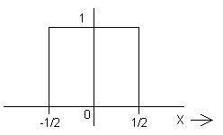
2. The rectangle function, |¯|(x).
|¯|(x) ≡ { 0; |x| > 1/2
(1/2; |x| = 1/2)
This piecewise continuous function is also known as the gate function. It is useful for "windowing" other functions, perhaps to represent the fact that in an experiment we take data only for a finite length of time. As our first function of finite width and finite integral, it raises two interesting questions.
---------------------------------------------------------------------------------------------------------------------------
(Aside on dimensions.)
H(x) has no finite width or scale. Its jump occurs in "zero" distance, and the two pieces of its domain are both semi-infinite. Since it only responds to the sign of its argument, that independent variable or parameter can have any dimensions at all. Such is not the case for |¯|(x). As physicists, we should have been struck immediately by the fact that the independent variable in its definition cannot be a physical length, since it is being compared with the dimensionless number 1/2. There is a great deal of convenience in using the dimensionless variables of mathematics, but we must remember to make the argument of |¯| explicitly dimensionless when working with physical variables. Thus if t stands for time, |¯|(t/[1 second]) is a window in time of width 1 second, while formally |¯|(t) is meaningless.
---------------------------------------------------------------------------------------------------------------------------
(Aside on normalization.)
We see that there are two adjustable parameters for this piecewise continuous function ‑‑ its height and its width. For the standard definition of this function and others like it, we will find it very convenient to observe two normalization conditions. Working in terms of the mathematician's dimensionless variables:
a) If the value of the function is non‑zero at x = 0, set it equal to one there. (H(x) is an
exception to this.)
b) If the integral of the function over the entire domain is non‑zero, set it equal to one. (This is
actually the more important of these two conditions.)
---------------------------------------------------------------------------------------------------------------------------
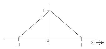
3. The triangle function, /\(x).
/\(x) ≡ { 1 ‑ |x| ; |x| < 1
0 ; |x| > 1
Notice that the full width of this function (the length of the x axis on which it is non‑zero) is actually 2, in order to meet both normalization conditions. Thus /\(x/X) has width 2X.
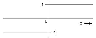
4. The signum function, sgn(x).
‑1; x < 0
sgn(x) ≡ { +1; x > 0
(0; x = 0)
Like H(x), sgn(x) has no width parameter and responds only to the sign of its argument. Thus there are no restrictions on the dimensions of its argument. It might seem logical to call this the "sign" function, but we need to communicate orally as well as in writing, and in this subject there is a very awkward homonym for that name!
As the plots of H(x) and sgn(x) should suggest to you, there is a simple connection between these two functions: sgn(x) = 2 H(x) ‑ 1. This raises the question of how many different piecewise continuous functions we should define and represent by distinct symbols ‑‑ at some point that process becomes counterproductive. We shall find that the uses for H and sgn are different enough to warrant thinking of them as different functions, yet in using each, we will often find it helpful to think of its relationship to the other. This is really a question of convenience and even taste. We have considerable freedom of choice, so we should be flexible in exercising it. The next two functions that I have chosen to define will not be useful in the long run, but they are particularly convenient for some introductory exercises. Giving them names and shorthand symbols will help us to think of them as complete entities, rather than just the results of some patchwork. That view is quite important for the approach that I wish to encourage.
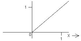
5. The ramp function, _/(x).
_/(x) ≡ { 0; x < 0
x; x > 0
Like H(x) and sgn(x), _/(x) also has no width parameter and hence can take an argument with dimensions. In place of the piecewise continuous definition above, we could just as well have written _/(x) ≡ x H(x). The expression x H(x) shows a very simple example of "plumbing with functions"; we have used multiplication by H(x) to chop off just the +x portion of the continuous function x and throw the rest away. This function has another simple connection to H(x). What is its derivative?
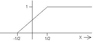
6. The ramped step function, _/¯(x).
0; x < ‑1/2
_/¯(x) ≡ { x + 1/2; |x| < 1/2
1; x > 1/2
This function does have a width parameter. Like |¯|(x) and /\(x), its argument must be made explicitly dimensionless when we use it for physical applications. If the step in H(x) seems too abrupt for your liking, then you have every right to think of H(x) as being "really" _/¯(x/X), with X too small for you to see. In fact I want to encourage you to take this view of any function with a discontinuity in its value; that perspective is central to the ideas of this subject. Of course if we cannot resolve the width of the ramp, then we cannot locate it with high precision either. Rather than being located symmetrically with respect to x = 0, it might "really" start at x = ‑X, or maybe at x = +2.93X. Perhaps the transition region "really" isn't even a straight segment, but something smoother that eliminates the angled corners found in _/¯(x). We don't know and we don't care, because as long as the width of the transition is smaller than the limits of resolution of our measuring apparatus, then we cannot know. For our purposes, all of these possibilities are covered concisely with the notation H(x). Whenever we use that notation, we should have it in the back of our minds that as far as we are concerned, it is just a shorthand for that infinite collection of possibilities. Do you buy this game? I hope so. Remember it!
(You may have noticed that _/¯(x) does not satisfy the first normalization condition on page 5, and neither does H(x). The definition of H(x) is well established in tradition, and for good reason. We will see some specific consequences of its deviating from that normalization condition, but they are much less troublesome than the awkwardness of defining H(x) as having value 2 when it is "on." The main use of _/¯(x) is as an approximation to H(x), and I chose to position the transition symmetrically about x = 0.)
B. Infinitely smooth functions.
In addition to piecewise continuous functions of the sort defined in the previous section, we will also find a good deal of use for functions with continuous derivatives of all orders. Some familiar examples of these infinitely smooth functions are the sinusoids and the positive integer powers of x, both of which are very useful in series expansions.
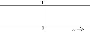
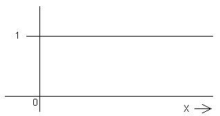
1. The unit function, 1(x) or x0.
1(x) or x0 ≡ 1; all x
Defining something that is "just a number" as a function of x, when it clearly has no dependence on that variable, may strike you as trivial, dumb, or just bizarre. Nevertheless the unit function is very useful in our pictorial manipulation of functions, for instance in relating H(x) and sgn(x) to each other. In situations where changes occur, we naturally tend to focus on the changes and ignore any DC or constant background terms, but they are there and can be important. Defining the unit function and manipulating it pictorially may reduce the likelihood of our overlooking such a term.
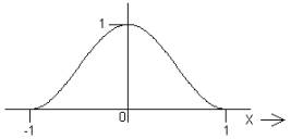 2.
The Gaussian function, exp(‑πx2).
2.
The Gaussian function, exp(‑πx2).
The important functional dependence here is exp(‑x2), and depending on the context in which you have encountered it before, you may know it in that form or perhaps as exp(‑x2/2σ2). Our definition satisfies the two normalization conditions given on page 5. It may seem awkward at this point, but later on we will realize some benefits from using this form.
3. The sinc function, sinc(x) ≡ (sin πx)/πx.
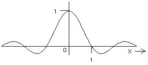
The important functional dependence here is (sin x)/x, and some people use that as the definition for "sinc." We include the factors of π to satisfy the normalization conditions, and again the benefits will be realized later. You are most likely to have run across this function as the diffracted amplitude from a single slit under Fraunhofer conditions. It may not surprise you then to hear that we shall find an intimate connection between this function and the rectangle function, which is the transmissivity profile for the single slit.
4. The complex exponential, exp(i2πs0x).
This is the single most important function in this course. Use every handle that you can find to get a good intuitive grasp of its meaning and the way that it works in various applications. Formal manipulations with this function can be done very quickly, and they yield powerful results, but we cannot afford to treat those manipulations as an algebraic black box from which the results emerge in some magical and mysterious manner. Such an approach could leave us in a state of sophisticated ignorance. We might become quite proficient at turning out results without having a sound basis for anticipating the behavior of those results and for checking their validity. The best remedy way to avoid that state of affairs is to develop a strong pictorial scheme to parallel and guide the algebraic treatment of the complex quantities.
---------------------------------------------------------------------------------------------------------------------------
(Aside on representing a complex function of a real variable.)
Clearly we have ventured into a new arena by allowing the dependent variable to take on complex values. A complex number can be thought of as an ordered pair of real numbers, which we call the real and imaginary parts:
z = (Re,Im) or Re + iIm,
where Re = the real part, and Im (without the i) = the imaginary part.
Similarly we can think of a complex function as an ordered pair of real functions. The famous formula credited to Euler represents the complex exponential in that form:
exp(i2πs0x) = cos(2πs0x) + i sin(2πs0x).
A nice justification for that relationship is provided by evaluating a power
series expansion on the exponential function, assuming only that the various
powers of the imaginary argument are to be dealt with according to the
relationship i2
= ‑1. This expansion
separates into two parts, the real one consisting of the even powers and
agreeing exactly with that for the cosine, and the imaginary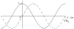 part consisting of the odd powers and agreeing with the series for the sine.
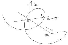
A standard way to represent the
ordered pair of real functions is to plot each one versus the independent
variable on the same set of axes, using a solid curve for the real part and a
broken curve for the imaginary part as shown here.
part consisting of the odd powers and agreeing with the series for the sine.
A standard way to represent the
ordered pair of real functions is to plot each one versus the independent
variable on the same set of axes, using a solid curve for the real part and a
broken curve for the imaginary part as shown here.
It is just because each member of the ordered pair for the complex exponential is a sinusoid that we shall find this function so useful in treating vibrations and waves. The sinusoidally varying physical quantities that we deal with are of course real, but it is often convenient to use a convention in which we represent those quantities by complex exponentials in our calculations and at the very end take the real part of the results. Initial discomfort over using a complex shorthand for real physical quantities can perhaps be eased by thinking that throughout the entire calculation, we "really" mean only the real parts, but the sooner you come to view the complex functions as having validity in themselves, the sooner you will tune into the considerable power of this approach. Right now would be a good time for you to review any materials that have exposed you to these ideas previously.
We can also represent complex numbers and functions in terms of magnitude and phase:
z = |z| exp(iφ) = |z| cos(φ ) + i |z| sin(φ ) = Re + iIm,
where |z| = (Re2+Im2)1/2 = (zz*)1/2 and φ = pha[z] = arctan(Im/Re). The complex exponential is particularly simple in this form; its magnitude is just the unit function, and its phase is directly proportional to x.
It
will be best if we think of both these representations as simply convenient ways
to handle a three‑dimensional situation in the two dimensions available on
paper. Try to develop the ability to move back and forth mentally
between them and the full three‑dimensional picture.
Keep it in mind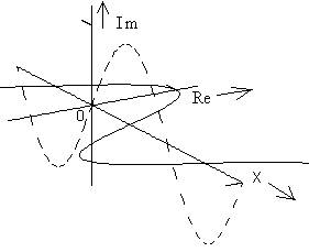 that the magnitude plot is just what we would obtain if the twisting figure in
three dimensions were flattened out by untwisting it, and the phase plot tells
us the amount of twist at any point along the x axis.
Similarly, the real and imaginary parts are just the projections of the
wire figure in three dimensions onto the (x, real) and (x, imaginary) planes,
respectively. Sometimes we will see this representation shown as those
projections in a 3‑dimensional perspective view.
that the magnitude plot is just what we would obtain if the twisting figure in
three dimensions were flattened out by untwisting it, and the phase plot tells
us the amount of twist at any point along the x axis.
Similarly, the real and imaginary parts are just the projections of the
wire figure in three dimensions onto the (x, real) and (x, imaginary) planes,
respectively. Sometimes we will see this representation shown as those
projections in a 3‑dimensional perspective view.
When I present a three‑dimensional perspective view of a complex function of one real variable, I often include "spokes" at a regular interval along the independent variable axis. (They are perpendicular to that axis.) This type of picture strongly suggests the representation in
terms of magnitude and phase,
which is the one that we will
find more useful in the long run.
---------------------------------------------------------------------------------------------------------------------------
(Aside on 2π or not 2π, i versus j.)
If you have done any work with complex exponentials before, you have probably been exposed to a different notation from that used here. For one thing, physicists tend to be lazy (or efficient) and leave out the explicit factor of 2π in the exponent. The appropriate parameter to use in that form is the propagation number k0 ≡ 2πs0. As shown in the figure at the beginning of this discussion, the wave number s0 has the simple significance that it is the reciprocal of the wavelength. Thus it is the exact spatial analog of the temporal frequency ν0 = 1/T, and at times I will refer to it as the spatial frequency. Its units could be inverse meters or inverse centimeters, for example, and just as with the temporal frequency, you might feel more comfortable inserting "cycles" as a placeholder to make it "cycles per meter" (or other appropriate unit of length). The propagation number k0 is the spatial analog of the angular frequency ω0 ≡ 2πν0, and it is quite advisable to think of it as being so many radians per meter, even though we will not be so quantitative as to work with numerical values for it. (Unfortunately some authors refer to k0 as the wave number. In that case you might want to mentally insert the adjective “angular.”)
We
shall find some real advantages in working with s0 rather than k0,
so I will emphasize the wave number at first. Later
on we can get a bit lazy and use k0, thinking of it as a convenient shorthand
for 2πs0. Similarly,
in translating between these two parameters it is convenient to think of s0
as just k0/2π
≡ k0. (That’s
my crude typographic attempt at “k-bar,” analogous to “h-bar” in quantum
mechanics.) I have put the subscript "0" on all the parameters
here because I am discussing the specific complex exponential shown in
the figure. Later we will find it
useful to let s be a continuous variable. Even
then, if we deal with one of these complex exponentials as a function in
the direct or x space, then there is just one specific value for s involved and
it should carry a subscript to indicate that fact.
Physicists tend to use i more than j to stand for the square root of ‑1, and the opposite is true for engineers. Also physicists tend to work on spatial problems involving waves more than do engineers, who typically focus on temporal and frequency descriptions of electrical or mechanical systems. When we define the Fourier transform and start using it, we shall find it essential to have one consistent convention for signs in the exponents. Thus it is awkward that a sinusoidal wave propagating in the + x direction is represented by cos 2π(s0x ‑ ν0t), which is the real part of exp(i2π[s0x ‑ ν0t]). I have opted to cope with this problem by fusing the convention most often used by physicists with that most often used by engineers. Thus for spatial work I will use exp( [i] 2πs0x), and for temporal work I will use exp( [j] 2πν0t), with the further convention that j = ‑i. (There is no difficulty in doing this. Just like any positive number, ‑1 has two square roots, which can be expressed as ±i or ±j. Since we have two symbols to represent the idea of a square root of ‑1, why not let them represent the two different roots?) For a full‑blown wave problem involving both space and time, I will then use
exp( [i] 2πs0x + [j] 2πν0t) = exp( [i] k0x + [j] ω0t)
to represent a wave propagating in the +x direction.
If you use the results of other authors, you will find that most of the time their notations agree with one half or the other of this strange mixed one, but you should never take that for granted. When physicists discuss vibrations, they often employ exp( [+i] ω0t), and I have occasionally seen engineers use exp( [‑j] ω0t). Always check to make sure that you know what convention is in use.
A good warning sign that you and an author are using different conventions is the appearance of exponential growth when there is no physical source of energy present, and you should be getting the usual exponential decay associated with damping. The fix in that case involves replacing erroneous complex quantities by their complex conjugates. If you have mixed some of your own expressions with those of the author, then you will have to examine them carefully to see which ones should be changed.
---------------------------------------------------------------------------------------------------------------------------
C. Other useful functions (a little plumbing).
The Heaviside step and the rectangle function are useful for chopping off a desired portion of a continuous function and eliminating the rest of it. These examples show H(x) used as a switch and |¯|(x) used as a window or gate. Both of the resulting piecewise continuous functions are useful enough to warrant giving them names for future reference.
1. The exponential wake, exp(‑x) H(x).
The exponential function exp(‑x) by
itself would cause some big problems
because of the way that it blows up as
x → ‑ ∞. Multiplying it by H(x) yields
a function which does not have that problem. It represents the way that this functional dependence actually appears in physical situations. Notice that even though this function is non-zero on a semi‑infinite domain segment, its integral is finite. Because of the presence of the H(t), this is another exception to the first normalization condition.
2. The Hanning pulse, 0.5(1 + cos πx) |¯|(x/2).
The first derivative of this function is
continuous everywhere. Its parameters
have been adjusted to satisfy the two
normalization conditions on page 5. In
some applications the discontinuities in
|¯|(x) troublesome. We could then use
/\(x) instead, so that at least the function itself is continuous. If /\(x) is not smooth enough for our purposes (because its first derivative has discontinuities), then we could turn to the Hanning pulse. This piecewise continuous function was named after Otto von Hann, who developed it as a smoothed window function for use in digital spectrum analysis.
D. Some basic operations.
The previous sections have defined quite a few useful functions, which you can think of as the raw materials for your new trade. Here are some tools with which you can start to manipulate them and put together some interesting structures.
1. Weighting: f(x) → a f(x).
This operation hardly seems to warrant a name ‑‑ it simply means scalar multiplication. Later on we shall find that it combines with another operation plus integration to yield the most important operation in this course. We shall allow the scalars to be complex, in which case we can think of weighting as a two part process:
a. multiplication by the real, positive |z|, and
b. rotation of the whole function through the angle φ = pha[z] about the x axis.
2. Shifting: f(x) → f(x ‑ x0).
This one can fool you if you are not
careful. If x0 > 0, then f gets shifted
to the right of its original location.
Here is one way to keep things straight.
Whatever behavior the original f had
at the origin, where its simple argument x was = 0 (in this case, hitting its maximum value), that same behavior will now be displayed at the new point where the fancier argument (x ‑ x0) is = 0, hence at x = x0. Notice the form I have given for the shifted function ‑‑ think of that as the standard one. If you are given something like f(x + a), it will probably be best to think of it (and maybe even rewrite it) as f(x ‑ [‑a]).
3. Flipping: f(x) → f(‑x).
This could also be called left‑right
inversion through the origin. There
is nothing very subtle here. It is one
special case of the next operation.
4. Rescaling (similarity transformation):
f(x) → f(x/X), with X real.
This one can also fool you if you
are not careful. It has the effect of
stretching out or compressing the
function along the x axis while leaving its general shape unchanged. This standard form is the one that should help you to keep things straight. Whatever the original f(x) did at a specific value for x (such as hit a peak, or pass through zero), the rescaled f(x/X) now does the same thing at X times that specific value for x. Notice that if X < 0, the rescaling includes a flip. Very often we will see a rescaling given in the form f(x) → f(ax), and that can be tricky unless we deliberately rethink it or rewrite it as f(x/[1/a]). Notice that the larger the |a|, the narrower the rescaled function will be.
5. Combinations of operations 2 ‑ 4.
If you are confronted with something like f([ax + b]/c), it can seem a bit formidable to try to visualize the plot of this function from a plot of the original f(x). By recasting the argument into the standard form
f(sgn(X)[(x-xo)/|X|]),
we can make that visualization quite straightforward. The value ‑1 or +1 for sgn(X) tells us explicitly whether or not there has been a flip. The new "center" of the function (location of the behavior that was originally at x = 0) is xo, and |X| is the factor by which the original f(x) has been stretched or shrunk horizontally.
One aspect of these combined operations which might seem backwards to you is the fact that the operation closest to the independent variable x is the one that has been performed most recently (last). The operation farthest from the independent variable is the one performed earliest (first). Each single operation (other than weighting) is just a careful SUBSTITUTION of something else for x alone, never for an expression involving x. Use the given standard form of the argument because it shows any flipping and/or rescaling being done first, and shifting last. The opposite order would be quite obscure, because flipping or rescaling after a shift changes that shift. On the other hand, a later shift does not alter the effects of an earlier flipping or rescaling.
E. Symmetries.
1. Even/odd.
An even function is one for which f(‑x) = f(x). Equivalently, we could say that an even function is invariant (left unchanged) under the flipping operation.
An odd function is one for which f(‑x) = ‑f(x). Thus flipping an odd function is equivalent to scalar multiplication by ‑1. We could also say that an odd function is invariant under the combined operation of flipping and weighting by ‑1: ‑f(‑x) = f(x).
2. Real/imaginary.
A real function is one for which f*(x) = f(x), so it is invariant under complex conjugation. Equivalently, its imaginary part = the zero function.
An imaginary function is one for which f*(x) = ‑f(x), so conjugation of such a function is equivalent to scalar multiplication by ‑1. Alternatively, an imaginary function is invariant under the combined operation of complex conjugation and weighting by ‑1. Of course the real part of an imaginary function is zero.
3. Hermitian/antihermitian.
A function is hermitian if it satisfies f*(x) = f(‑x). Thus complex conjugation of a hermitian function is equivalent to flipping it. One could also say that a hermitian function is invariant under the combined operations of flipping and complex conjugation. The real part of a hermitian function is even, and its imaginary part is odd.
An antihermitian function satisfies f*(x) = ‑f(‑x), or equivalently, it is invariant under the three combined operations of conjugation, flipping, and multiplication by ‑1. Its real part is odd, and its imaginary part is even.
F. Symmetry operations.
Any function can be decomposed into two parts according to any of the three symmetries in the previous section. That is, it can be expressed as the sum of even and odd parts,
the sum of real and (i times) imaginary parts, or the sum of hermitian and antihermitian parts:
f(x) = E[f(x)] + O[f(x)] = Re[f(x)] + i Im[f(x)] = Herm[f(x)] + Anti[f(x)].
In the following decompositions, notice how the expression for evaluating any part of f(x) relates to the operation or the combination of operations under which that part is invariant.
Taking even/odd parts.
E[f(x)] = [f(x) + f(‑x)]/2
O[f(x)] = [f(x) ‑ f(‑x)]/2
Taking real/imaginary parts.
Re[f(x)] = [f(x) + f*(x)]/2
Im[f(x)] = [f(x) ‑ f*(x)]/2i
(Remember that the imaginary part of a complex number is real.)
3. Taking hermitian/antihermitian parts.
Herm[f(x)] = [f(x) + f*(‑x)]/2
Anti[f(x)] = [f(x) ‑ f*(‑x)]/2
Many useful applications for these symmetry considerations will become apparent once we have defined the Fourier transform. Paying attention to symmetries is an important part of being truly in control of a calculation. It can save you a lot of detailed work, and it also provides a quick check on the results.