Waves à la Fourier Introduction: Background material on vibrations and waves, using DPGraph.
I. A debate on the use of figures -- some relevant quotes and my position.
“No diagrams will be found in this work.” Joseph Lagrange, Mechanique Analytique.
“Pictures after all may be suitable only for very young children; Lagrange dispensed entirely with such infantile aids when he composed his analytical mechanics.” Eric Temple Bell, Men of Mathematics, p. 400.
--------------------------------------------------------------------------------------------------------------
“Gauss once called mathematics ‘the science of the eye.’” E. T. Bell, p. 407. (Source?)
“Many scientists know Fourier theory not in terms of mathematics, but as a set of propositions about physical phenomena. Often the physical counterpart of a theorem is a physically obvious fact, and this allows the scientist to be abreast of matters which in the mathematical theory may be quite abstruse....The present work began as a pictorial guide to Fourier transforms to complement the standard lists of pairs of transforms expressed mathematically. It quickly became apparent that the commentary would far outweigh the pictorial list in value, but the pictorial dictionary of transforms is nevertheless important, for a study of the entries reinforces the intuition....” Ronald N. Bracewell, The Fourier Transform and Its Applications, p. 2.
The two positions represented here seem to reflect a difference in fundamental concerns: formal, detailed proofs on the one hand, and an organized structure of understanding on the other. The latter is useful not only for consolidating our current knowledge but also for suggesting new directions to pursue. For about 125 years, engineers, physicists, and applied mathematicians followed the lead of Joseph Fourier in using a mathematical description of nature that is well suited to the conditions found in a laboratory. Laurent Schwartz finally succeeded in justifying it formally in 1948. It’s a good thing that those who worked on real problems arising in technology and the study of nature hadn’t waited for the pure mathematicians to catch up!
This study will make use of some convenient graphical tools for examining the detailed behavior of vibrations and waves. The static, two-dimensional pictorial dictionary in Bracewell’s textbook made a tremendous advance with its concise representation of piecewise continuous functions and their Fourier transforms. DPGraph and MATLAB go much farther by providing the user with hands-on controls for manipulating the parameters of kinetic images. Complex functions of a real variable and some other images are essentially three-dimensional, and the ability to view them from several different directions helps us to understand them better. I make no apologies for using such “infantile aids” as these. They will help you to become familiar with some very powerful mathematical ideas for dealing with vibrations and waves.
II. Basic definitions and some details of elementary wave behavior.
There are major problems regarding the use of precise terminology when we discuss vibrations and waves. A few outright misnomers have become well established. Introductory treatments of waves often place undue emphasis on idealized special cases without the use of any qualifying adjectives. This approach can lock us into thinking in terms of those unrealistic examples when we encounter a problem in real life. We begin with an attempt to clarify some basic definitions.
Vibration -- back-and-forth motion of an object about its rest position, or variation of some property of a system about its equilibrium value. There is NO IMPLICATION OF REPETITION in the use of this term. In practice we focus much of our attention on repetitive or periodic vibrations, and sinusoidal motion will play an especially important role in our work, but those are SPECIAL CASES. Vibrations at different locations are often coupled by waves.
Wave -- a disturbance that travels from one location to another without an actual transfer of matter between those locations. Mechanical waves such as sound, surface waves on water, and earthquake waves require a material medium, but electromagnetic waves propagate very well in a vacuum. Again there is NO IMPLICATION OF PERIODICITY in the use of this term. Energy and momentum are transported by waves. (Under extreme conditions, when nonlinear effects become noticeable, matter is able to “surfride” on waves. We do not deal with those situations.)
Linearity -- a condition under which superposition is valid. Different vibrations may be present simultaneously in the same object or system. If they do not interact with each other, we have a choice of handling them all together or dealing with them separately and then adding them up -- superimposing them. A similar statement can be made for waves found in the same region of a medium or empty space. A “divide and conquer” approach that treats components separately is very powerful; for that reason we limit our study to linear vibrations and waves in this course.
“Waveform” -- an unfortunate misnomer that should more logically be called the “history of a vibration.” It shows the dependent variable plotted vertically versus TIME as the independent variable. Vibratory motion may occur simultaneously at different locations, but a waveform displays the time record at one location only. If we are interested in the behavior of a wave, we may want to work with a single snapshot of it, or perhaps a sequence of frames from a movie or a video recording. These images have POSITION as their dependent variable. They are NOT WAVEFORMS -- even though that would be a logical name for them! This misnomer is so well established that we cannot go against traditional usage.
Our discussion becomes more concrete at this point with the introduction of the first DPGraph figure. Click on this link to open the file WavePulse.dpg. In the toolbar at the top of the screen, click on “Scrollbar.” Click the circle to the left of “A variable” and then “OK.” Find the scrollbar on the right side of the screen and place the cursor right on the box with the up arrow, at the top of the bar. Click repeatedly on that box to view successive frames in a movie of an asymmetric pulse wave that travels to the right. Notice that the independent variable (position along the medium) is labeled as “y,” and the dependent variable is “z.” Time runs backwards if you click repeatedly on the down arrow box at the bottom of the scrollbar. You can jump eight frames at a time by clicking in the scrollbar just adjacent to either arrow box. Return the value of “a” to zero (position the slider at the bottom) before you go to the next step.
What at first appears to be just a two-dimensional display is actually a succession of slices or sections of a three-dimensional image. Use both the down and right arrows on the keyboard -- just a few taps for each -- until you see the outline of an empty box at an oblique angle. The y axis should be toward the front (bottom of the screen), the z axis should be vertical, and the new x axis should be on the left, coming out toward you. (If you overshoot in using these keys and get confused, return to the original orientation by hitting the Home key.) Now as you increase the “a” variable by clicking the box at the top of the scrollbar, you will see the succession of movie frames advancing obliquely. A continuous record of those frames and intermediate wave images is left behind as a surface, colored blue on the top and pink underneath. The complete figure, with “a” at its maximum value, would be a good one to use while trying out the arrow controls to change its orientation. You can also see the blue/pink surface partially through the white screen of the last frame by selecting “Surface transparency” under the Scrollbar options and increasing its value. This looks a little better if you select a white background. Play with the Page Up, Page Down, and Home keys on the keyboard as well. Be sure that you set “a” at its maximum value, to show the complete surface, before you go on to the next step.
The x axis in this display corresponds to time. (Unfortunately we are not able at this time to select our own labels for the three axes.) In the oblique view, you might have noticed that a shape very much like that seen in each movie frame was traced out in the x,z plane (y = 0) as you advanced time by increasing “a.” This plot is the waveform for the particle at y = 0. You can focus your attention more easily on that waveform by selecting “B variable” under the Scrollbar options. One click on the up arrow box then separates that waveform from the rest of the blue/pink surface. Additional clicks do the same for other locations that are progressively farther along the y axis. Notice that they all have the same shape, but each one is just shifted in time by its propagation delay, Δt(y)= y/c, where c is the wave speed. Also notice the left-right reversal of the triangles in these waveforms compared to the triangles in the movie frames. This reversal is common to all waves that propagate to the right along the position axis.
[It appears that we have c = 1 in these dimensionless coordinates, so the triangles in the two types of plot have the same width. This is a convenient relationship, and it is guaranteed by working in the natural units of length for the wave disturbance -- the “wave-second,”or an appropriate power of 10 times that. For electromagnetic waves the basic unit is the light-second = 3x10⁸ m; for sound it would be the sound-second = 340 m, the distance traveled by sound in one second; and so on.]
AN IMPORTANT DISCLAIMER! We have tried to be careful to avoid associating the term “wave” too strongly with any idealized special cases of that very broad category. The example used here has some special behaviors of its own. Notice that it travels to the right without any change in its shape. If you have ever launched a pulse wave on an electrical power cord or a garden hose to unhook it from a snag, you might have noticed that it gets weaker and spreads out as it progresses. We also observe that many waves start off with fairly sharp corners but become more rounded with time. None of these realistic behaviors disqualifies the motion from being called a wave disturbance.
III. Extracting some math from this special case.
Usually waves are introduced by deriving the differential equation for the motion of an idealized limp string or perhaps a simple model of a sound wave inside a pipe. Then solutions are presented and shown to satisfy the equation. Let’s reverse the process and work backwards from our idealized solution to find an equation that it satisfies. The essence of the behavior that we have examined is that the wave disturbance can be represented in the form z = f(y - ct) ≡ f(α), where c is the speed with which the disturbance advances to the right and f is an arbitrary function -- not just the particular lopsided triangle that we have chosen. Using the chain rule, it is easy to see that ∂z/∂t = -c ∂z/∂y, independent of the specific form of f(α). Hence we have “a wave equation” that is satisfied by the general expression for the observed behavior.
An odd aspect of this equation is that it only allows waves to propagate to the right, in the direction of increasing y. We know that waves can travel in either direction on a string or in a pipe, so we should also deal with disturbances of the form g(y + ct) ≡ g(β) which travel to the left at speed c, again with g(β) arbitrary. A different “wave equation” that is satisfied by g is clearly ∂z/∂t = +c ∂z/∂y. The string or pipe is a single object, and there is no real difference in the manner that a wave propagates in either direction, so there should be a single differential equation that is satisfied by both forms of solution. We obtain that equation by going to the next order of partial derivatives: ∂2z/∂t2 = c2 ∂2z/∂y2. This is the simple wave equation which is satisfied by traveling waves of unchanging shape that move in either direction. You may be more used to seeing it written in the form ∂2z/∂y2 - (1/c2)∂2z/∂t2 = 0. Superposition applies, because each partial derivative enters in only to its first power (linearity). A general solution is then z = f(y - ct) + g(y + ct), with no special relationship between the functions f and g unless we are trying to satisfy a boundary condition, such as that imposed by a reflector at some location.
A detail that bothered mathematicians for quite some time was the question of just how arbitrary the shapes of f(α) and g(β) could be if they are to satisfy this second-order partial differential equation. A seemingly obvious requirement is that they should each have second second-order partial derivatives, in other words that those derivatives should be finite everywhere. Let’s look into that aspect of the particular shape for f(α) that we have used here -- the asymmetric triangle.
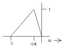
First we need to represent it mathematically. The skill of moving back and forth between a figure and its mathematical representation is one that I hope you will learn to use quickly and accurately. It’s both fun and very useful. Notice that we must develop different expressions for different segments of the independent variable axis. This is an example of a piecewise continuous (PC) function.
Write the expression for f(α) in each of the four segments shown here. (4 segments? yes) Find df/dα in each segment, and sketch it. Now do the same for d2f/dα2. Are you sure about your result? Check it by integrating to see if you get back to your df/dα. You should find that you are facing a dilemma here. PONDER IT!
![]()